Welcome to the GPS-X Slideshow! This slideshow presents many of the
powerful features of GPS-X, and demonstrates how a GPS-X layout is
developed from start to finish. Please take a few moments to work through
the slideshow; alternatively, you may wish to wait for all of the images
to load and then print out a hard copy of the slideshow so that you may
review it at your leisure.

Slide 1: The GPS-X Drawing
Board

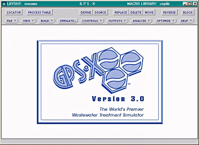
This is GPS-X's main window. It contains GPS-X's main menu bar (the
buttons labelled "FILE", "VIEW", "BUILD", etc., are drop-down menus which
each contain several GPS-X commands); it also contains buttons which bring
up other windows (the "LOCATOR" and "PROCESS TABLE" buttons) as well as
buttons which modify the drawing mode (the "REPLACE", "DELETE", "MOVE",
"REVERSE", and "BLOCK" buttons).
The large area below this row of buttons is GPS-X's "drawing
board"; the layout of the treatment plant to be modelled is created here.
[top][next][end]

Slide 2: Starting a GPS-X Layout

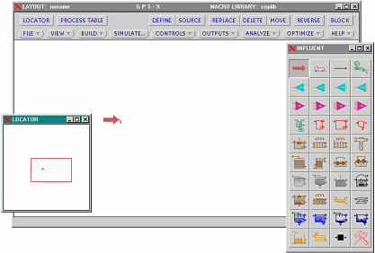
For this slideshow, we will be building a layout representing a
treatment plant with both primary and secondary treatment; the secondary
treatment will be carried out using the activated sludge process, using
two parallel liquid trains.
The first step is to bring up the GPS-X Process Table; this is a
window which contains all of the objects available in GPS-X (see Slide 3
for a labelled close-up of the Process Table). From the Process Table,
objects can be selected and placed on the drawing board. In this slide, we
have placed an influent object on the drawing board.
The "LOCATOR" window can be used to select an area of the drawing
board for viewing. Here we have selected an area large enough to hold our
completed layout.
[top][prev][next][end]

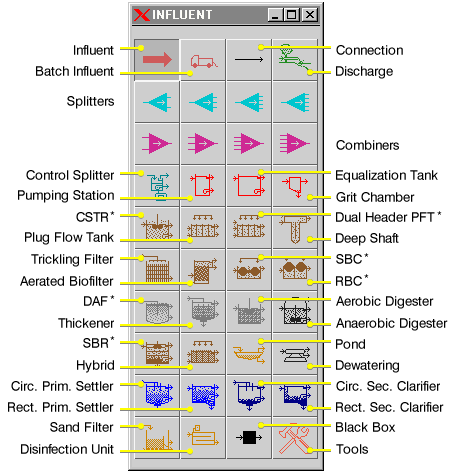
Slide 3: The Process Table


The GPS-X Process Table contains allows easy access to all of the
objects supported by GPS-X. To place one of these objects on the drawing
board, the user simply selects the desired object with the mouse, and then
clicks on the desired location of that object in the drawing board.
*The acronyms used in this figure are defined below:
- CSTR: Continuous Stirred Tank Reactor
- PFT: Plug Flow Tank
- SBC: Submerged Biological Contactor
- RBC: Rotating Biological Contactor
- DAF: Dissolved Air Flotation
- SBR: Sequencing Batch Reactor
[top][prev][next][end]

Slide 4: Continuing the Layout

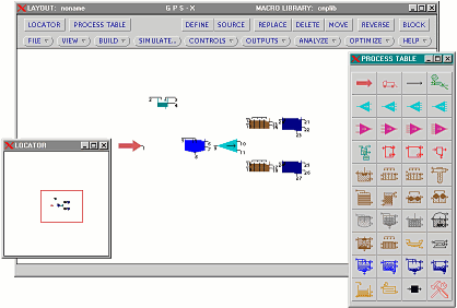
Several objects have been added to the layout. At the far left is
the influent object, which represents the influent entering the plant. To
the right of the influent object is a pump object; this will allow
by-passing of the plant during very high influent flow conditions. To its
right is a combiner object, followed by a primary clarifier. Two liquid
trains have also been added, each containing a plug-flow reactor object
(representing an aeration tank) and a secondary clarifier.
Several objects have been added to the layout. To the right of the
influent object at the far left is a pump object; this will allow
by-passing of the plant during very high influent flow conditions. To its
right is a primary settler, followed by a splitter object. Two liquid
trains have also been added, each containing a plug-flow reactor object
(representing an aeration tank) and a secondary clarifier.
[top][prev][next][end]

Slide 5: Completing the Layout

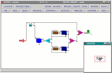
The layout of the plant has been completed: several objects have
been added, and the connections between the objects have been defined --
all accomplished with just a few clicks of the mouse. The only new object
type is the right-most object in the layout, which is an effluent object
representing the effluent discharge point. The new objects are at the far
right in the layout: an effluent object representing the effluent
discharge point, and two combiner objects.
[top][prev][next][end]

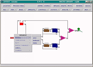
Slide 6: Defining the Models


Once the layout has been completed, it is necessary to define which
models are to be used for the objects in the layout. For example, the user
can choose from one of three possible models for the influent object:
- asm2: for influents characterized using COD and suspended
solids as the main components
- bodbased: used when COD data is not available
- states: useful only if a full influent characterization has
been performed and the state variables have been calculated manually
[top][prev][next][end]

Slide 7: Defining the Models (continued)

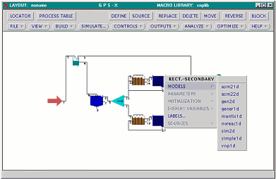
The model for the secondary clarifier in the first (topmost) liquid
train is being defined. The user can choose from several settling models,
including reactive and non-reactive models, as well as one-dimensional and
two-dimensional models.
[top][prev][next][end]

Slide 8: Setting the Parameters

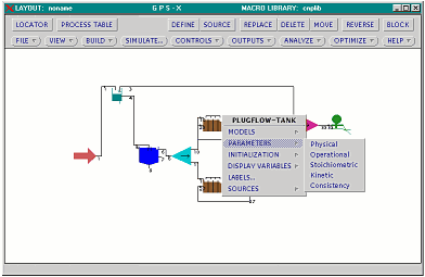
After models have been assigned to each of the objects, the next
step is to define the necessary parameters. For the plug flow reactor
object, the following types of parameters can be set:
- the physical parameters, which include the volume and size of
the tank, as well as the number of "cells" into which it is divided;
- the operational parameters, which include parameters
controlling the aeration of the reactor, aeration control (P/PI/PID), as
well as the recycle between cells in the tank;
- the stoichiometric parameters, which include ratios such as
COD to suspended solids;
- the kinetic parameters, which define rate constants for the
various reactions.
- the stoichiometric parameters, which include ratios such as
COD to suspended solids;
- the kinetic parameters, which define rate constants for the
various reactions; and
- the consistency parameters, which define alarm bounds for
certain variables in each unit process object.
[top][prev][next][end]

Slide 9: Setting the Parameters (continued)

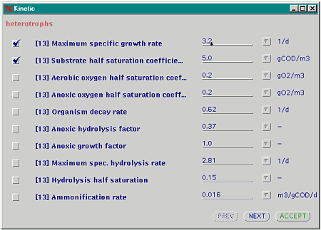
A form such as this one allows the user to enter the model
parameters. This form allows the kinetic parameters of the plug flow
reactor to be set; additional parameters can be accessed using the "NEXT"
button. The values shown here are the default values for the kinetic
parameters of the plug flow reactor object.
The check marks in the squares to the left of the first two
parameters indicate that we intend to manipulate these parameters during
the course of a simulation. (The check marks are placed here as an example
only; we do not actually want to manipulate these parameters for this
example.)
[top][prev][next][end]

Slide 10: Building a Controller

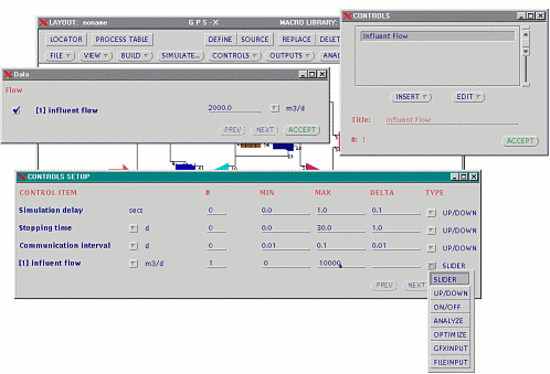
In this example, we want to be able to control the influent flow
rate as the simulation progresses. The required steps are:
- Place a check mark beside the influent flow variable in the influent
object;
- Create a new control window, and call it "Influent Flow" (since this
is the first control we have created, it has the ID of 1);
- In the "CONTROL SETUP" window, assign the influent flow variable to
the control window with an ID of 1, make it a slider control, and give
the slider minimum and maximum values of 0 and 10000 m3/day,
respectively.
In addition to slider controls, incremental
up/down controls and on/off controls can be defined.
[top][prev][next][end]

Slide 11: The Completed Controller


Once the controller has been defined, it can be displayed with the
"SHOW" item of the "CONTROLS" menu.
This slider allows the user to manipulate the flow between 0
m3/day and 10,000 m3/day; this is done by dragging
the handle of the slider with the mouse. The number to the left of the
slider represents the current value of the slider.
[top][prev][next][end]

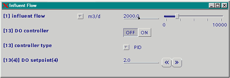
Slide 12: Controller Types


This slide shows the different types of controls that can be
defined. (Please note, however, that the controls shown here are not used
in this example, with the exception of the influent flow slider).
On/off controls are often used for activating and deactivating
automatic controllers; the on/off control shown in this slide controls the
operation of the automatic dissolved oxygen controller.
The "controller type" control is a drop-down control. Available
options for the "controller type" variable are P, PI, and PID; this
control allows the user to select from these options.
The "DO Setpoint" control is an up/down control; the value of the
dissolved oxygen setpoint can be incremented or decremented by clicking on
the left and right arrows, respectively.
[top][prev][next][end]

Slide 13: Building a Graph


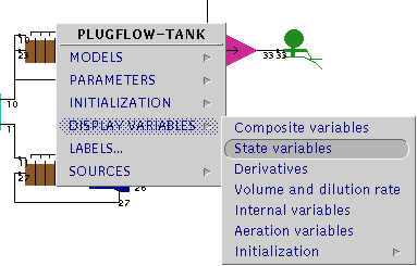
Each object has a number of "display variables" that can be placed
on various types of graphs. Here, we wish to place the dissolved oxygen
profile on a graph, so we need to display the "state variables" dialog
(since dissolved oxygen is a state variable).
[top][prev][next][end]

Slide 14: Building a Graph (continued)

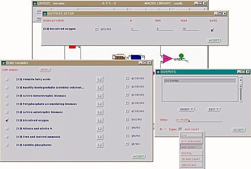
The steps required to complete our graph of the dissolved oxygen
profile are:
- Place a check mark beside the dissolved oxygen display variable in
the "state variables" dialog of the plug flow reactor object.
- In the "OUTPUTS" dialog, create a new graph window (using the
"INSERT" button), assign it the name "DO Profile", and make it a bar
graph. Since this is the first graph window we have created, it is
assigned an ID of 1.
- In the "OUTPUTS SETUP" window, assign the dissolved oxygen variable
to the graph window with an ID of 1 (the graph window we have just
created), and enter the minimum and maximum bounds for the y-axis of
this variable.
By placing a check mark in the "SAVE" box in the
"OUTPUTS SETUP" window, the simulation results for that variable will be
saved to a file; these results can then be imported into any spreadsheet.
Also note that there are several types of graphs available to the
user; these are:
- X-Y: Standard line graphs with linear x and y axes.
- X-Y SCROLLING: X-Y graphs with a "scrolling" x-axis -- the
time span shown on the graph is fixed, but the upper and lower bounds
increase as the simulation progresses.
- BAR CHART: Bar charts showing the values of an array variable
(for example, dissolved oxygen in a multi-tank plug flow reactor).
- DIGITAL: Numeric values of variables.
- 3D BAR CHART: Three-dimensional bar charts showing the values
of three-dimensional array variables.
- GREYSCALE: Like the 3D BAR CHART, these graphs display the
values of three-dimensional array variables; the values are represented
as varying shades of grey.
[top][prev][next][end]

Slide 15: The DEFINE Command


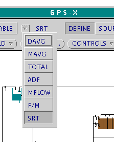
GPS-X's DEFINE command can be used to define parameters which are
not related to any particular object or model, but rather are "plant-wide"
in scope. One such variable which is used frequently in wastewater
engineering is the solids retention time (SRT), which is selected above.
Other variables which can be defined with this command are:
- DAVG: defines a variable which represents the daily average of the
specified GPS-X variable.
- MAVG: defines a variable which represents the moving average of the
specified GPS-X variable.
- TOTAL: defines a variable which represents the integral over time of
the specified GPS-X variable.
- ADF: defines a variable which represents the filtered value of the
specified GPS-X variable. An advanced custom filtering method, called
the Adaptive Data Filter, is used to filter the data.
- MFLOW: defines a variable which represents the mass flow rate of the
specified GPS-X variable.
- F/M: defines a variable which represents the food-to-mass ratio for
the specified objects.
[top][prev][next][end]

Slide 16: Compiling the Model


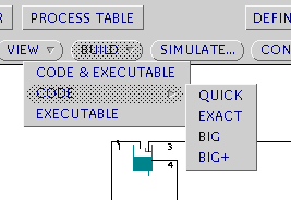
Once the layout has been completed and the desired controls and
displays have been defined, it is necessary to compile the model in order
to simulate the plant. Normally, this can be done in one step by clicking
on the "BUILD" button; however, in certain special situations the code and
the executable files must be generated separately, as shown above.
Normally, for models of moderate size, the compilation step takes
only one or two minutes.
[top][prev][next][end]

Slide 17: Starting the Simulation/Defining a
Scenario

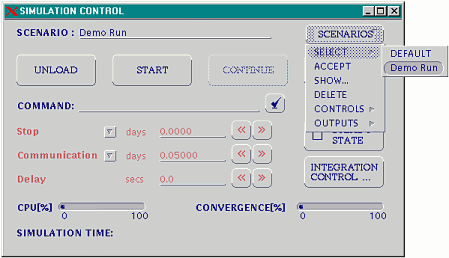
Once the model has been compiled, simulations can be run from the
"SIMULATION CONTROL" window. "Scenarios" can also be defined from this
window. In GPS-X, a scenario is simply a list of commands that are
recorded when you make changes to the object data entry forms.
Saving a scenario stores these commands for later retrieval; running the
scenario involves the playback of these instructions.
Here, we have defined a "Demo Run" scenario, in which we have
modified the influent flow rate and the wastage flow rate in the plug flow
reactors.
[top][prev][next][end]

Slide 18: Running the Simulation to Steady-State

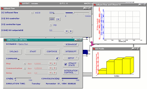
Often, it is desired to run the model to steady-state before
performing dynamic simulations. In GPS-X, this is done by checking the
"STEADY STATE" box and then starting the simulation. Here, the
steady-state simulation has achieved 100% convergence, as indicated by the
"CONVERGENCE" bar in the lower-right corner of the "SIMULATION CONTROL"
window.
[top][prev][next][end]

Slide 19: Running a Dynamic Simulation

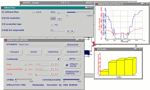
This slide shows a one-day simulation in progress. The graph in the
upper-right corner shows the influent flow rate (in red) as well as the
effluent suspended solids (in blue). The histogram in the lower-right
corner shows the instantaneous dissolved oxygen profile in one of the plug
flow reactors.
The influent flow rate has been modified from its initial value by
manually adjusting the position of the slider in the upper-left corner.
[top][prev][next][end]

Slide 20: Comparing Simulation Results to External
Data

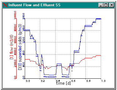
Suppose that you had both influent flow rate data and effluent
suspended solids data for a real plant. In order to calibrate the model,
you would need to be able to compare the simulation's output variables of
interest (here, effluent suspended solids) for a simulation which uses the
same time-varying inputs as your real plant (here, influent flow rate).
In GPS-X, this is easily accomplished: the influent flow rate
controller can be defined as a "file-input" type controller, meaning that
it takes data from an external data file. Effluent suspended solids data
can be displayed automatically alongside the simulation results; the data
is plotted as plusses ("+") while the simulation results are continuous
lines.
The case in this slide is obviously synthetic; it has been created
from the saved results of a previous simulation, which was then re-run
with slight modifications to the secondary clarifier's settling
parameters. However, it demonstrates the ease with which GPS-X can be used
to develop calibrated models.
[top][prev][next][end]

Slide 21: The ANALYZE Tool


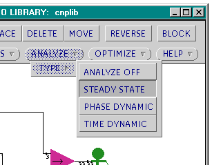
Often, it is necessary to determine the sensitivity of the model's
results to fluctuations in certain parameters -- for example, to obtain a
measure of the error in the model's predictions. This can be easily
accomplished with the GPS-X's ANALYZE Tool. Here, we will set up a
steady-state sensitivity analysis of the mixed liquor suspended solids to
the wastage flow rate from the plug flow reactor.
[top][prev][next][end]

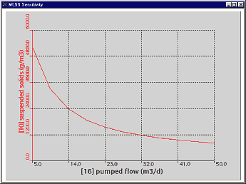
Slide 22: MLSS Sensitivity Analysis


This slide shows the results of the completed sensitivity analysis.
Graphs of this type can be used to determine the amount of wastage
necessary to achieve a desired level of MLSS.
[top][prev][next][end]

Slide 23: The GPS-X OPTIMIZER


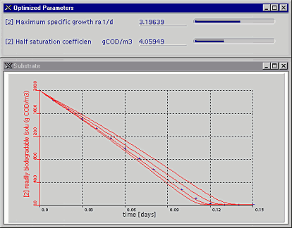
The GPS-X OPTIMIZER can be used to automate many of the tedious
tasks required to calibrate a model. In this slide we are simultaneously
optimizing the value of two parameters which control the kinetics of the
biological reactions in a batch reactor. The OPTIMIZER will find the
values of the parameters which results in the best possible fit betwen the
simulated soluble substrate values and those supplied in an external data
file.
[top][prev][end]

The End!

This is the end of the GPS-X slideshow. While we have covered many
of GPS-X's features, GPS-X has many more powerful features that make it
the best wastewater treatment plant simulator available. Examples of
features not covered in this slideshow include:
- Model customization
- Report generation
- On-line capability
- Dynamic parameter estimation
- Automated respirogram evaluation
- Maximum likelihood estimation
- MATLAB® support
- Multivariable control design with GMITM
- More...
| 
![]()
![]()

![]()
![]()

![]()
![]()

![]()
![]()

![]()
![]()

![]()
![]()

![]()
![]()

![]()
![]()

![]()
![]()

![]()
![]()

![]()
![]()

![]()
![]()

![]()
![]()

![]()
![]()
